Keccacheck: towards a SNARK friendly Keccak

Proving hash computations is the bread and butter of modern proof systems. Take storage proofs as an example. Let's say we run a DeFi lending protocol, based on funds that are held in Ethereum accounts. Participants in the protocol might want to prove that they own at least N USDC without revealing their exact balance or who they are. Our work on this problem started in collaboration with VLayer, whose need for efficient storage proofs served as the initial motivation.

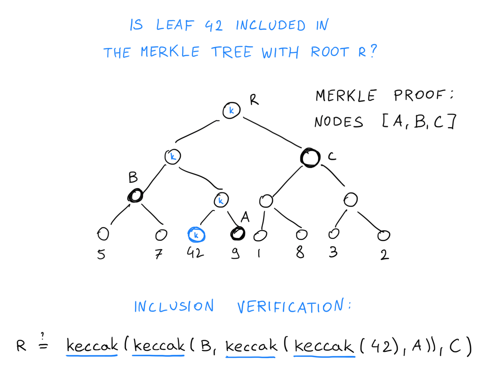
To do this, a ZK circuit must be constructed that takes the account balances and the Merkle proof path in the Ethereum state trie. The circuit’s computation first hashes each account’s data to generate a leaf node, then iteratively hashes up the Merkle path, ultimately verifying that the calculated root matches the true root node for that block.

The issue with this approach is that Ethereum uses Keccak-256 hashes inside its Merkle trie. Keccak is designed to be fast in hardware, and hence uses bitwise operations, but these are much, much slower inside an arithmetic circuit.

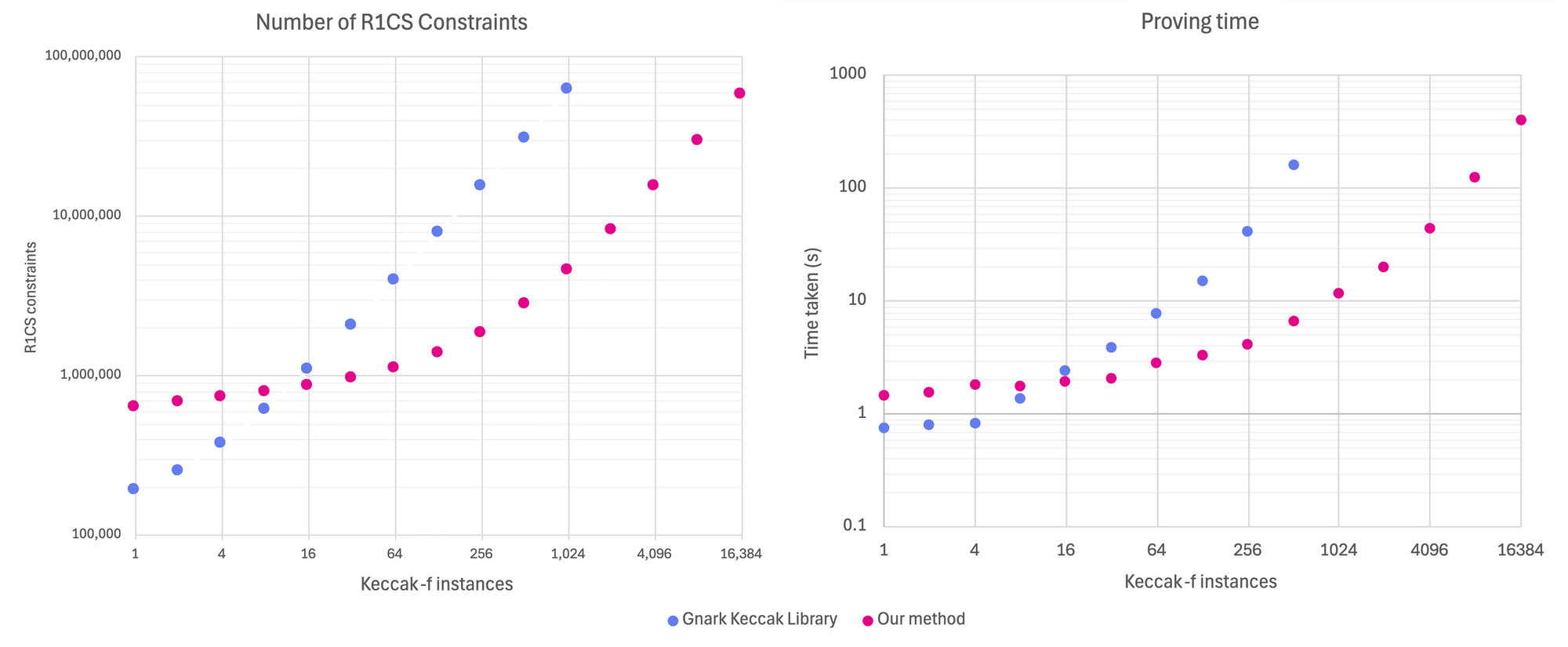
Our approach to proving Keccak hashes scales well beyond what’s possible with directly computing hashes in Gnark, and offers over 10x improvement for batch sizes of at least 512 hashes.

Main approach

The keccak-f permutation iterates in stages (called iota, chi, pi, rho, and theta). Each keccak-f stage operates on a state that contains 25 64-bit words. At each stage of the permutation we perform bitwise operations on each word of the state to produce the next value of that state. The main trick is that we are able to represent each of the state words—and all the bitwise operations to permute their values—as polynomials.

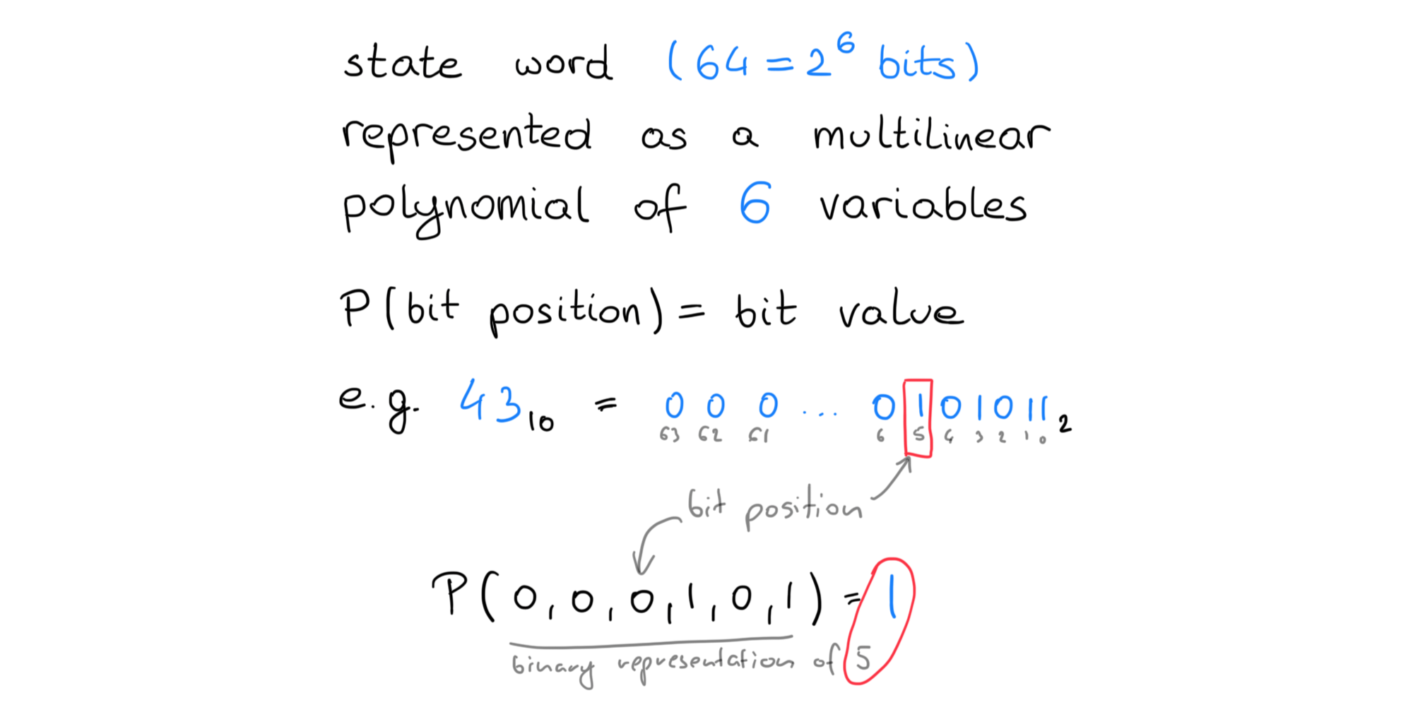
To represent a keccak-f state word as a polynomial, we will perform a multilinear extension (MLE) of its bit array. To do so, we use an “eq” polynomial that, on boolean vectors, outputs 1 if both inputs are the same, and 0 otherwise. For non-boolean input vectors, it outputs some other, well-defined, value. We can then express any state element \(A[i][j]\) evaluated on field elements as the following (\(k\) is the index of a bit in a 64-bit word):

$$A_{ij}(\alpha) = \sum_{k\in\{0, 1\}^6} \text{eq}(\alpha, k) \cdot A[i][j][k]$$

It is easy to see that this form is correct when \(\alpha\) is boolean; because both sides are multilinear polynomials that agree on \(2^{\text{(num vars)}}\) points, they must be identical everywhere in the field.

We can also express bitwise operations using arithmetic operations. For example, an exclusive-or operation can be represented as \(\oplus(a, b) = a + b - 2 ab\). It is easy to verify that—for boolean inputs—this will only evaluate to 1 if either \(a\) or \(b\) are equal to 1, but not both. For all other field elements the value is also well-defined.

A few of the canonical expressions for bitwise operations:

The question is how we can use these bitwise polynomials to bridge between the steps of the permutation. Imagine we have a very simple xor stage that takes two words, represented as polynomials, \(P\) and \(C.\) The result of this operation will be a new word \(P’\). To verify if xor was performed correctly, the verifier could plug in all \(2^6 = 64\) boolean assignments into \(P, P’, C\) and manually check the following:

Obviously, this is extremely time-consuming for the verifier. Instead, we can represent \(P, P’, C\) as MLEs, and sum over all possible inputs. Using the Schwartz-Zippel lemma, we'll test a single random (non-boolean!) vector \(\alpha\) in our field \(\mathbb{F}\) and be very confident that—if results agree—we indeed have identical polynomials and that xor was computed correctly.

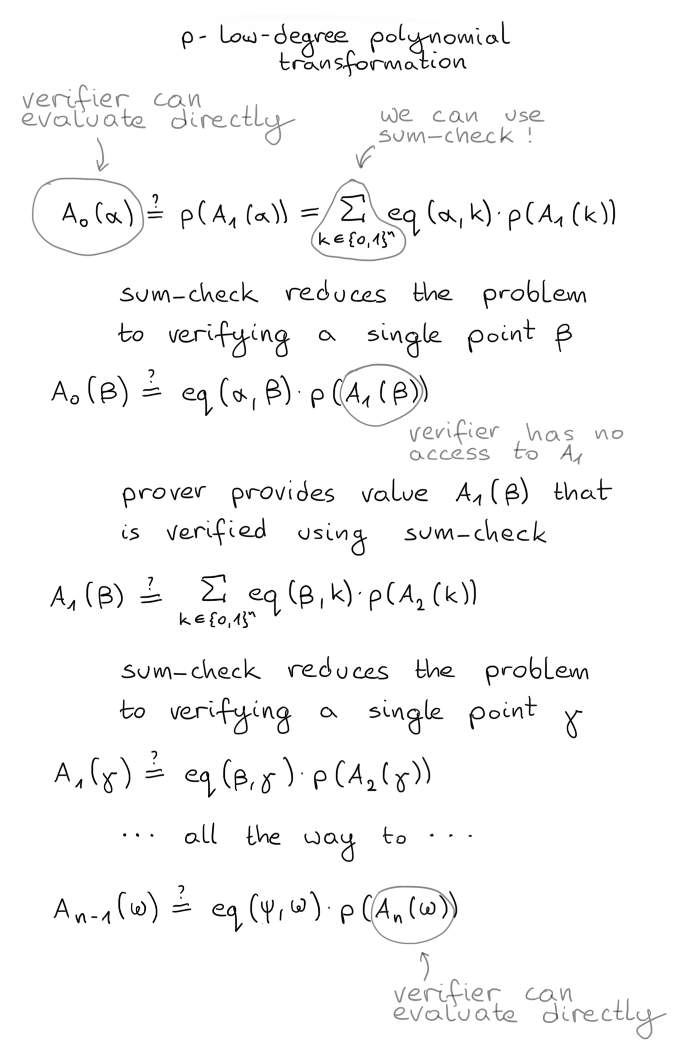
We still need to figure out what to do with \(2^6\) terms under the sum. Luckily, the sum-check protocol allows us to provide the verifier with a sum of all boolean evaluations of a polynomial (evaluations for all bits of our state), and prove that said sum is correct without the verifier needing to re-do the work. It does this by reducing the verification of that sum to the verification of one polynomial evaluated at a random point.

We can see how, if we can express our current claim as a sum of the boolean evaluations of the previous layer, we will be able to reduce that to a single claim about the previous layer.

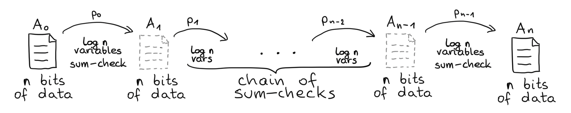
Let’s go back to the polynomial of a single state word. The verifier picks a random point and asks the prover to evaluate the polynomial at that point. Let’s call that point \(\alpha\) and the polynomial \(p_{i,j}\) where \(i\) is the stage of the keccak-f function that we are at and \(j\) is the word index of the state. We are now able to do reduce that claim on \(p_{i,j}(r_0)\) to a claim on \(p_{i-1, j}(r_1)\), one layer closer to the input.

Once we have moved a layer closer to the input, we can start the process again. We can continue in this vein until we reach the inputs; the verifier has access to the inputs so can verify the evaluation claims directly.

Batching

We can prove multiple keccak-f instances at once by use of batching. The core idea is that when we double the number of instances being proved, we need only add 1 extra variable to the MLE polynomial of each state evaluation claim. The intuition for this is that we assign each instance a binary index \(g\); it’s easy to see that for each extra bit in the index, we can accommodate 2x more instances. The summation claim adapts naturally to this setting. Remember that we define each claim \(A_{ij}(\alpha)\) as: $$A_{ij}(\alpha) = \sum_{k \in \{0,1\}^6} eq(\alpha, k) \cdot A[i][j][k]$$ To support batching, we can add variables and define it in the same way. If we let the number of instances be \(n\), instance number \(g = k_{6..(6 + log(n))}\), bit position \(b = k_{0..6}\), we get: $$A_{ij}(\alpha) = \sum_{k \in \{0,1\}^{6 + \text{log}(n)}} eq(\alpha, k) \cdot A_g[i][j][b]$$

Optimisations and tricks

Readers familiar with GKR might already recognize the idea of chaining sum-checks layer by layer. Our approach has a few significant changes from the original GKR:

• No predicate function: by writing polynomials by hand, we can directly index into the correct nodes from the previous layer, skipping the need to evaluate complex predicates.
• Not propagating data through each layer: traditionally, GKR circuits are only allowed to read data from the previous layer. This is especially wasteful for Keccak, where certain steps often modify only 5 helper bitvectors on the side. By manually writing all polynomials, we can refer directly to other states in layers beyond the previous.
• Linear combination of state elements: GKR layer sizes are always a power of two. In cases where we propagate 25 state elements, we essentially waste 7/32 of the available space. We fix that by working on each state element separately (and since each element is u64, it aligns with GKR perfectly) and taking a random linear combination of these elements for cheap verification. There is a small price to pay as a result: at each step we need to send a bit more data to the verifier (namely, evaluations at the selected challenge for each state element), but our benchmarks show the tradeoff to be well worth it.

Not directly related to GKR, we also employ a few clever tricks to make things even faster:

• Mixture of closed-form and interpolated polynomials (with at most 6 variables): The performance of the verifier is tied to having access to closed-form polynomials (i.e. given as a formula) whenever possible. It inserts a random challenge into the formula, evaluates it once, and is then done. However, a closed form for bitwise rotation is tricky—the formula is so complex that it’s actually cheaper to remember all evaluations on binary inputs and use interpolation to calculate values at the random challenge. This works because we always rotate exactly 64 bits (i.e. in other words, we interpolate a MLE of only 6 variables)
• Changing base for even more efficient xor: to better arrange terms in our polynomials and reduce the number of multiplications, it can sometimes help not to think in binary zeros and ones and the usual \(xor(x, y) = x + y - 2xy\) formulation. Instead, we can use a different basis where \(-1\) represents a true value, and \(1\) represents false. In this representation, xor is a simple multiplication, with all the benefits like being able to factor out a common element from a string of xors. Let \(x\) be the traditional 0, 1 base, and \(\hat{x}\) a 1, -1 base. It’s easy to see that \(\hat{x} = 1 - 2x\).

Finally, using an efficient sum-check implementation helps a lot, too. We’ve used ProveKit as an inspiration, and hand wrote the folding steps for great multithreading performance. ProveKit includes other cool tricks such as evaluating polynomials at infinity to save on some multiplications.

Why we needed recursion

In our protocol we faced 2 issues.

1. The protocol as described is not zero-knowledge. The verifier is sent both the outputs and the inputs of the permutation function. Imagine a case where we want to prove a Merkle commitment has been correctly calculated, but we don’t wish the verifier to know the values being committed. The protocol as is does not support such zero-knowledge operation.
2. Proof sizes in this model are large. Specifically we need to send \(2929 + 552 * n\) field elements. Even at lower numbers of \(n\), this amounts to hundreds of KB.

We address both problems by recursing once: we prove the verification of the first proof. SNARKs can prove the correct execution of any computation—including the verifier’s computation itself. By wrapping the original verifier inside a SNARK, we achieve:

• Zero-Knowledge: The SNARK hides the inputs to the permutation function, so the verifier learns nothing beyond the statement’s truth.
• Compact Proofs: Groth16 proofs are very small, replacing the original proof with a much smaller one.

Performance and security

The reason why our technique scales so well in the number of constraints is that sum-check verification scales linearly in the number of variables. This means that verifying a state transition costs \(O\big(\text{log(number of hashes)}\big)\) constraints. The beginning and end of the protocol, that directly evaluate polynomials, cost a linear amount of constraints, but those are the only linear factors. Contrast this to directly hashing in the circuit where the entire algorithm scales linearly.

Security in our protocol follows from the security of the sum-check protocol. Our protocol satisfies round-by-round soundness, meaning it is secure under the Fiat Shamir transform, assuming a sufficiently secure hash function (the technical term being “a correlation-intractable hash”).

Summary

Our approach is a novel take on the sum-check and GKR protocols. By designing a system specialized for Keccak proving, our team was able to achieve drastic speedups compared to existing generic high-level solutions. This can be compared to hand coding assembly for particularly intensive parts of an application. For users who need to prove Keccak hashes at scale, such as storage proof providers, our solution can offer over 10x improvement when proving batches of at least 512 hashes. For really high-traffic situations, the improvement is even larger, scaling well beyond what’s possible with direct Keccak hashing in gnark.

If your company is interested in reducing compute or gas costs, please reach out to Reilabs. We would be happy to help!

Hope you have enjoyed this post. If you'd like to stay up to date and receive emails when new content is published, subscribe here!